Linear Regression Implementation from Scratch

Dive into Deep Learning · §2.4

Linear regression implemented from first principles
model · loss · optimizer · training loop.

We know the answer before we start

Motivation

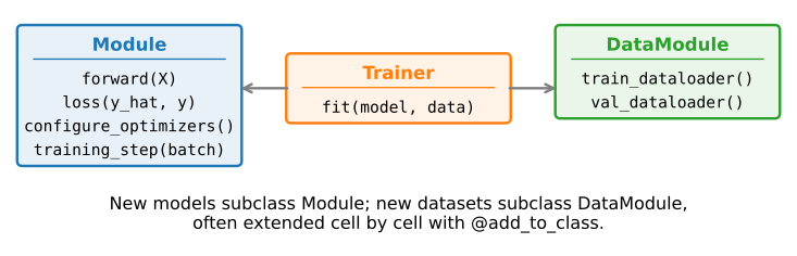
The implementation has four explicit pieces: a model (w, b, forward), a loss, an optimizer, and the training loop driving them, each slotted into the Module / Trainer / DataModule scaffold of the object-oriented-design section.

Because we manufactured the data (the synthetic-regression-data section, noise \sigma = 0.01), we can check a correct implementation against known targets. We compare two quantities: a loss near the expected noise floor \sigma^2/2 = 5\times10^{-5}, and parameters returning to \mathbf{w}^* = [2, -3.4], b^* = 4.2.

The Model

parameters and the forward pass

Parameters: small random w, zero b

The Model

We need parameters before we can optimize them. Draw w from a tiny Gaussian, set b to zero:

class LinearRegressionScratch(d2l.Module):
    """The linear regression model implemented from scratch."""
    def __init__(self, num_inputs, lr, sigma=0.01, rngs=None):
        super().__init__()
        self.save_hyperparameters(ignore=['rngs'])
        rngs = nnx.Rngs(d2l.get_key()) if rngs is None else rngs
        self.w = nnx.Param(
            rngs.params.normal((num_inputs, 1)) * sigma)
        self.b = nnx.Param(jnp.zeros(1))

PyTorch’s requires_grad=True is the flag that matters: it tells autograd to track w and b so gradients can flow back from the loss (JAX tracks via its grad transformation, TensorFlow via GradientTape, MXNet via attach_grad). For this single linear layer, a small initialization works (exercise 1); symmetry breaking only matters once we stack layers.

Forward pass: one matrix-vector product

The Model

The model is an affine map: multiply the feature matrix by the weights and add the bias.

\hat{\mathbf{y}} = \mathbf{X}\mathbf{w} + b

@d2l.add_to_class(LinearRegressionScratch)
def forward(self, X):
    return d2l.matmul(X, self.w) + self.b

\mathbf{Xw} is a vector, b a scalar; broadcasting adds b to every entry.

This affine map is the complete linear-regression architecture. Later networks compose affine maps with nonlinearities and other structured operations.

Loss & Optimizer

what to minimize, and how

Loss: mean squared error

Loss

Squared error per example, averaged over the minibatch:

\ell(\hat{y}, y) = \tfrac{1}{2}\,(\hat{y} - y)^2

@d2l.add_to_class(LinearRegressionScratch)
def loss(self, y_hat, y):
    l = (y_hat - d2l.reshape(y, y_hat.shape)) ** 2 / 2
    return d2l.reduce_mean(l)

The \tfrac12 makes the gradient just \hat{y}-y; averaging (not summing) keeps the step size independent of batch size.

The gradient, by hand

Loss

What is it that the backward pass will compute? For one example \ell = \tfrac12(\hat{y}-y)^2 with \hat{y}=\mathbf{w}^\top\mathbf{x}+b, the chain rule gives:

\frac{\partial \ell}{\partial \mathbf{w}} = (\hat{y}-y)\,\mathbf{x}, \qquad \frac{\partial \ell}{\partial b} = (\hat{y}-y).

Averaged over a minibatch \mathcal{B}, that is the entire gradient the optimizer consumes:

\nabla_{\mathbf{w}} L = \frac{1}{|\mathcal{B}|}\sum_{i\in\mathcal{B}}(\hat{y}^{(i)}-y^{(i)})\,\mathbf{x}^{(i)}, \qquad \nabla_{b} L = \frac{1}{|\mathcal{B}|}\sum_{i\in\mathcal{B}}(\hat{y}^{(i)}-y^{(i)}).

The gradient is the error-weighted input: a large residual \hat{y}-y gives a proportionally large weight gradient in the direction of \mathbf{x}. This is exactly what the backward pass fills in and what the SGD step subtracts.

A transformable loss

Loss · JAX

NNX modules own their parameters, while nnx.value_and_grad exposes the trainable part of that object graph to JAX. The loss can therefore call the model directly without manually threading a parameter pytree:

@d2l.add_to_class(LinearRegressionScratch)
def loss(self, y_hat, y):
    l = (y_hat - d2l.reshape(y, y_hat.shape)) ** 2 / 2
    return d2l.reduce_mean(l)

NNX separates graph structure from array state at transformation boundaries, preserving the pure computation required by jit and grad.

Minibatch SGD as an Optax transform

Optimizer · JAX

Optax expresses an optimizer as two pure functions, init (empty state) and update (gradients to the increment -\eta\,\mathbf{g}), wrapped in a GradientTransformation:

class SGD(d2l.HyperParameters):
    """Minibatch stochastic gradient descent."""
    # The key transformation of Optax is the GradientTransformation
    # defined by two methods, the init and the update.
    # The init initializes the state and the update transforms the gradients.
    # https://github.com/deepmind/optax/blob/master/optax/_src/transform.py
    def __init__(self, lr):
        self.save_hyperparameters()

    def init(self, params):
        # Delete unused params
        del params
        # Return an EmptyState *instance* (an empty NamedTuple, hence a valid
        # pytree) -- not the class -- so this hand-rolled optimizer is
        # JIT-traceable just like any optax GradientTransformation.
        return optax.EmptyState()

    def update(self, updates, state, params=None):
        del params
        # NNX's Optimizer applies these updates to its model's parameters.
        updates = jax.tree_util.tree_map(lambda g: -self.lr * g, updates)
        return updates, state

    def __call__(self):
        return optax.GradientTransformation(self.init, self.update)

Training

the loop that ties it together

One minibatch: four steps, in order

Training

Each minibatch update consists of four steps:

Forward + loss, while recording the computation for differentiation.
Clear the old gradients before the backward pass writes new ones.
Backward to fill each parameter’s gradient.
Update the parameters, outside the gradient graph.

Clear gradients before the backward pass so they do not accumulate across minibatches. Keep the update outside the graph so it is not differentiated.

Training loss approaches the noise level

Training · results

Model, synthetic dataset, Trainer; ten epochs at learning rate 0.03:

model = LinearRegressionScratch(2, lr=0.03)
data = d2l.SyntheticRegressionData(w=d2l.tensor([2, -3.4]), b=4.2)
trainer = d2l.Trainer(max_epochs=10)
trainer.fit(model, data)

The fit call drives the four-step loop over every minibatch and plots both losses live.

Both curves flatten near \approx 5\times10^{-5}, consistent with the \sigma^2/2 noise contribution. Validation closely tracks training in this run, as expected for 2 parameters fitted to 1000 points (the generalization section).

Compare fitted and generating parameters

Training · results

The synthetic generator specifies \mathbf{w}^*=[2,-3.4], b^*=4.2. The result:

print(f"error in estimating w: "
      f"{data.w - d2l.reshape(model.w[...], data.w.shape)}")
print(f"error in estimating b: {data.b - model.b[...]}")

error in estimating w: [ 0.00044107 -0.00051808]
error in estimating b: [0.00095987]

Off by a few 10^{-4} at most. Exact recovery needs linearly independent features and is not the everyday goal (deep models have many equally good parameter settings, and we care about accurate prediction), and accurate prediction is normally the primary objective. Here the fitted parameters are close to the generating values.

Recap

Wrap-up

A Module for linear regression is just __init__, forward, loss, configure_optimizers.
The gradient is the error-weighted input, (\hat{y}-y)\,\mathbf{x}, what backward deposits and SGD consumes.
The optimizer is a ten-line minibatch SGD.

Training is one loop per minibatch: forward and loss, clear the old gradients before backward, then update outside the graph.
Both targets met: loss on the 5\times10^{-5} noise floor, \mathbf{w}, b recovered to \sim10^{-4}.

Next, we express the same model with framework components and then introduce additional losses, optimizers, and regularizers.