Concise Implementation of Linear Regression

Dive into Deep Learning · §2.5

The same model, the concise way
batteries-included layers, losses, and optimizers replace the hand-rolled parts.

From hand-rolled to high-level

Motivation

Last section we wrote every piece by hand: the weight vector, the forward pass, the squared error, the update step.

Those pieces are so universal that frameworks ship them, tuned and tested. We swap each one for its built-in counterpart:

Layer replaces w, b · loss replaces our squared error · optimizer replaces the update loop.

By hand	Built-in
w, b	a layer
MSE math	a loss
update step	an optimizer

01

The Model

a single linear layer

The layer already is the model

The Model

What we hand-rolled as w, b, and a matrix–vector product, every framework ships as a fully connected layer: each input wired to the one output: exactly the picture of linear regression.

The layer owns its parameters. We no longer allocate them, initialize them, or even know their shapes ahead of time.

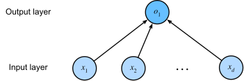
One fully connected layer with a single output is linear regression.

One layer, with explicit sizes and randomness

The Model

nnx.Linear(num_inputs, 1, rngs=rngs) defines the complete linear model. NNX has no lazy mode, so we state the input width and hand the layer an explicit RNG stream — and its parameters exist, on the module, as soon as the constructor returns:

class LinearRegression(d2l.Module):
    """The linear regression model implemented with high-level APIs."""
    def __init__(self, num_inputs, lr, rngs=None):
        super().__init__()
        self.save_hyperparameters(ignore=['rngs'])
        rngs = nnx.Rngs(d2l.get_key()) if rngs is None else rngs
        self.net = nnx.Linear(
            num_inputs, 1, kernel_init=nnx.initializers.normal(0.01),
            rngs=rngs)

The JAX interface makes both shapes and randomness explicit. The weights then live on the module, just as in the other frameworks.

The forward pass delegates to the layer

The Model

forward just calls the layer. All the matrix–vector arithmetic we wrote by hand now lives inside it:

@d2l.add_to_class(LinearRegression)
def forward(self, X):
    return self.net(X)

02

Loss & Optimizer

framework implementations of the remaining components

Loss: built-in mean squared error

Loss & Optimizer

The framework’s MSE replaces our hand-written squared error:

@d2l.add_to_class(LinearRegression)
def loss(self, y_hat, y):
    return d2l.reduce_mean(jnp.square(y_hat - y))

It omits the \tfrac{1}{2} factor we used by hand, and averages over the minibatch by default.

Configure minibatch SGD with an optimizer object

Loss & Optimizer

The update loop becomes a single optimizer object, handed the parameters and the learning rate:

@d2l.add_to_class(LinearRegression)
def configure_optimizers(self):
    return optax.sgd(self.lr)

The same optim/Trainer family also gives momentum, Adam, and more by changing the optimizer configuration.

03

Training

the same training interface applies

The Trainer uses the same model interface

Training

Our Trainer, Module, and DataModule from the object-oriented-design section don’t care that the model is now a built-in layer.

The training loop is identical to the from-scratch version.

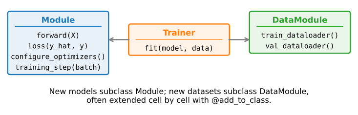
Fit: same data, same curve, a fraction of the code

Training

Same synthetic data, same ten epochs, same fit call as the linear-regression-from-scratch section:

model = LinearRegression(2, lr=0.03)
data = d2l.SyntheticRegressionData(w=d2l.tensor([2, -3.4]), b=4.2)
trainer = d2l.Trainer(max_epochs=10)
trainer.fit(model, data)

The two implementations use the same model, loss, data, and update rule; only the component implementations differ.

Where the parameters live now

Training · parameters

The parameters now belong to the layer rather than appearing as self.w and self.b, so get_w_b accesses them through net:

@d2l.add_to_class(LinearRegression)
def get_w_b(self):
    return self.net.kernel[...], self.net.bias[...]

w, b = model.get_w_b()

print(f'error in estimating w: {data.w - d2l.reshape(w, data.w.shape)}')
print(f'error in estimating b: {data.b - b}')

error in estimating w: [-2.6226044e-05 -1.8382072e-04]
error in estimating b: [0.00037479]

As in the linear-regression-from-scratch section, the generating values are \mathbf{w}^* = [2,-3.4] and b^* = 4.2. The fitted parameters are within a few 10^{-4} of them, and the built-in components implement the same computations.

Summary

Wrap-up

• From scratch showed what happens; concise uses the framework components typical of applications.
• A single layer stands in for w, b; a built-in loss and optimizer replace the rest.

• The Module / Trainer / DataModule scaffold is unchanged; only the model’s internals got shorter.
• Same minibatch loop, same convergence: ~5 lines of model code, error order 10^{-4}.