@nnx.jit
def _ppo_step(policy, opt, obs, act, adv, logp_old, mask, epsilon,
              entropy_coef, use_clip):
    def loss_fn(policy):
        logp_all = jax.nn.log_softmax(policy(obs), axis=-1)
        logp = jnp.take_along_axis(logp_all, act[:, None], -1).squeeze(-1)
        rho = jnp.exp(logp - logp_old)
        surr = jnp.where(use_clip, jnp.minimum(
            rho * adv, jnp.clip(rho, 1 - epsilon, 1 + epsilon) * adv),
            rho * adv)
        entropy = -(jnp.exp(logp_all) * logp_all).sum(-1)
        loss = -(mask * (surr + entropy_coef * entropy)).sum() / mask.sum()
        return loss, (rho, logp, entropy)
    (_, (rho, logp, entropy)), grads = nnx.value_and_grad(
        loss_fn, has_aux=True)(policy)
    opt.update(policy, grads)
    n = mask.sum()
    return ((mask * (jnp.abs(rho - 1) > epsilon)).sum() / n,
            (mask * (logp_old - logp)).sum() / n, (mask * entropy).sum() / n)

def ppo_epochs(ac, batch, adv, logp_old, epsilon, num_epochs,
               entropy_coef=0.01, use_clip=True):
    """num_epochs clipped-surrogate passes on one frozen batch; returns
    [num_epochs, 3] numpy diagnostics: fraction of ratios outside the
    band, approximate KL, mean policy entropy."""
    size = 1 << max(6, (len(adv) - 1).bit_length())
    mask = jnp.asarray((np.arange(size) < len(adv)).astype(np.float32))
    obs, act, adv, logp_old = (_pad(np.asarray(x), size) for x in
                               (batch.obs, batch.act, adv, logp_old))
    step = nnx.cached_partial(_ppo_step, ac.policy, ac.opt_pi)
    return np.array([step(obs, act, adv, logp_old, mask, epsilon,
                          entropy_coef, use_clip)
for _ in range(num_epochs)])Parameter Space versus Policy Space
One parameter, two actions (example due to Joshua Achiam), two updates of the same size \Delta\theta = 2:
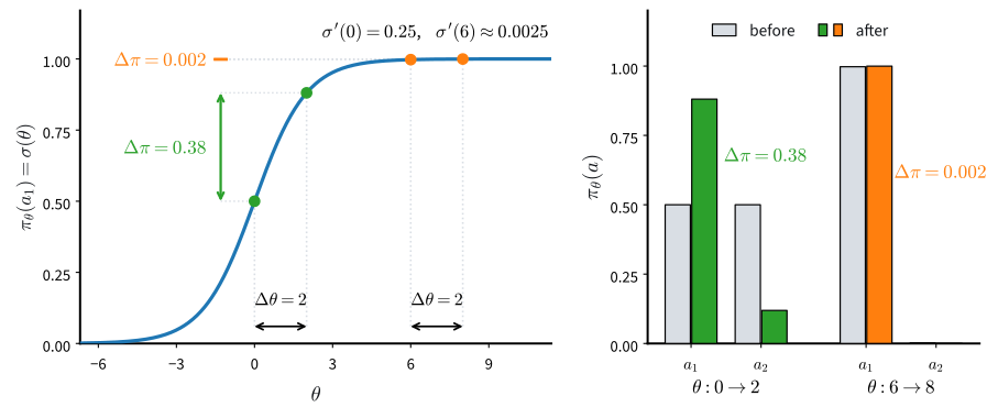
\sigma'(0) = 0.25 against \sigma'(6) \approx 0.0025: no learning rate is right in both regions. One oversized step near indifference throws the policy into saturation, scores vanish, and the on-policy data is collected by the broken policy: the run is over. Capping the step in \theta caps the wrong quantity.
TRPO: a Bound, then a Constraint
J(\theta) \geq J(\theta_{\text{old}}) + \bar L(\theta) - \frac{4\gamma A_{\max}}{(1-\gamma)^2} \max_s D_{\text{KL}}\big(\pi_{\theta_{\text{old}}} \Vert \pi_\theta\big)
Here \bar L is the population surrogate under the old policy’s discounted occupancy, and \bar L(\theta_{\text{old}})=0 exactly; its sampled estimate need not be zero. Increasing this lower bound guarantees monotonic improvement in J. Practical TRPO replaces the maximum statewise divergence by a sampled mean KL constraint over visited states and solves the resulting approximation with second-order optimization. The practical constraint is a proxy rather than the bound displayed above.
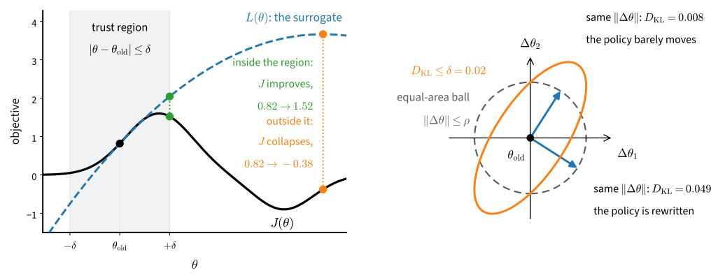
For small policy changes, KL divergence induces the Fisher metric, so the corresponding steepest-ascent direction is the natural gradient. This is another instance of the geometry-dependent norms discussed in :numref:sec_muon.
The Clipped Objective
L^{\text{CLIP}} = \frac1n\sum_{i,t} \min\!\big(\rho\hat A,\ \text{clip}(\rho,1-\epsilon,1+\epsilon) \hat A\big)
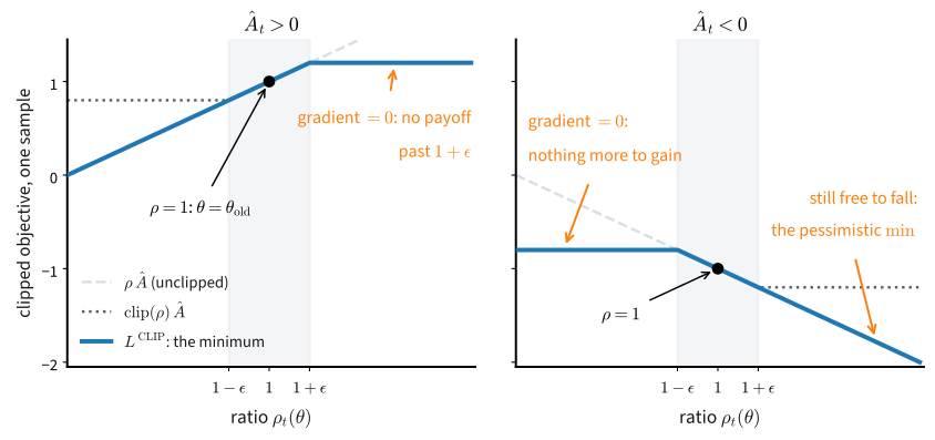
When a ratio crosses the clipping boundary in the direction that would improve the sampled objective, that sample contributes zero gradient beyond the boundary. Changes that worsen the objective remain unclipped. This construction resembles a trust-region penalty but provides no monotonic-improvement guarantee.
The Ablation: Eight Seeds, Clip On and Off
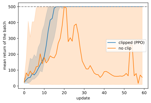
Both variants use the same batches and 20 optimization passes. At least half of the unclipped seeds collapse to returns near 9, whereas every clipped seed reaches the task ceiling. Roughly 5% of ratio evaluations activate the clip. The individual failing seeds vary between runs, but the failure frequency is consistent in this experiment.
Training Diagnostics
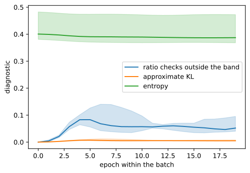
entropy: 0.64 over the first five updates, 0.26 over the last five- In these runs, KL divergence and clipping events are concentrated in the first optimization epochs for each batch; clipping limits subsequent drift.
- During training, entropy decreases from about 0.65 to 0.25 nats. The entropy bonus slows this decrease, as discussed in :numref:
sec_regularized.
Policy Drift within a Batch
Because the likelihood ratios are importance weights, their effective sample size provides a diagnostic of weight concentration:
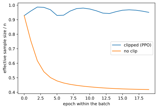
after 20 epochs the batch is worth 95% (clipped (PPO)) vs 42% (no clip) of its 136 stepsWith clipping, the likelihood ratios remain nearly uniform over the chosen number of epochs. Without clipping, their effective sample size falls to half the batch or less. This weight-only diagnostic does not account for advantages, sample dependence, or mismatch in the state distribution.